Lineage Note
1921-2026
Ralph Bown to RF Chronometric Interferometry
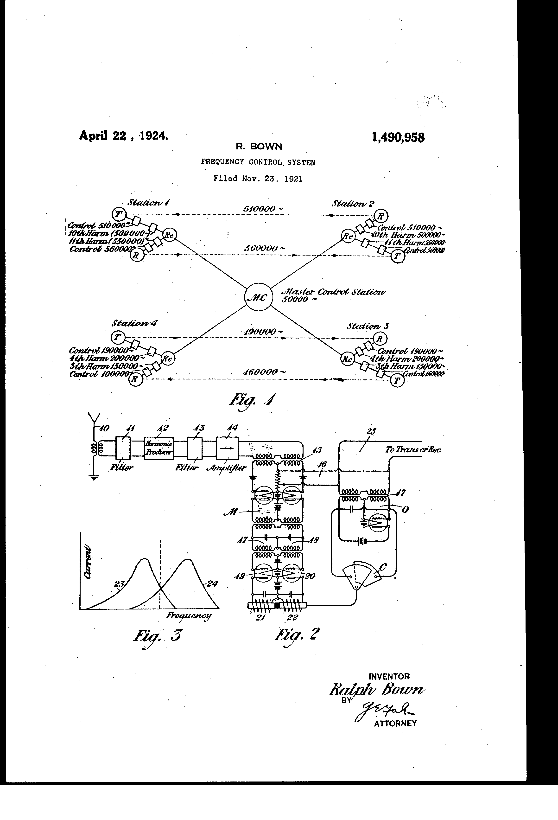
Driftlock Choir extends an established engineering lineage. In US1490958A (filed 1921, granted 1924),
Ralph Bown described a master station transmitting a frequency reference while subordinate stations
derived beat frequencies against local oscillators for control and synchronization.
The same physical mechanism appears in modern timing infrastructure: satellite-disciplined references
in GPS-era systems and carrier-phase comparison in RF synchronization research. Driftlock Choir applies
this method at 5.8 GHz to resolve sub-picosecond timing through phase estimation.
Timeline: 1924 master-reference beat-note control → 1970s GPS timing references → 2026
RF carrier-phase femtosecond simulation record.
Citation: Ralph Bown, Frequency-Control System, US1490958A, granted April 8, 1924.
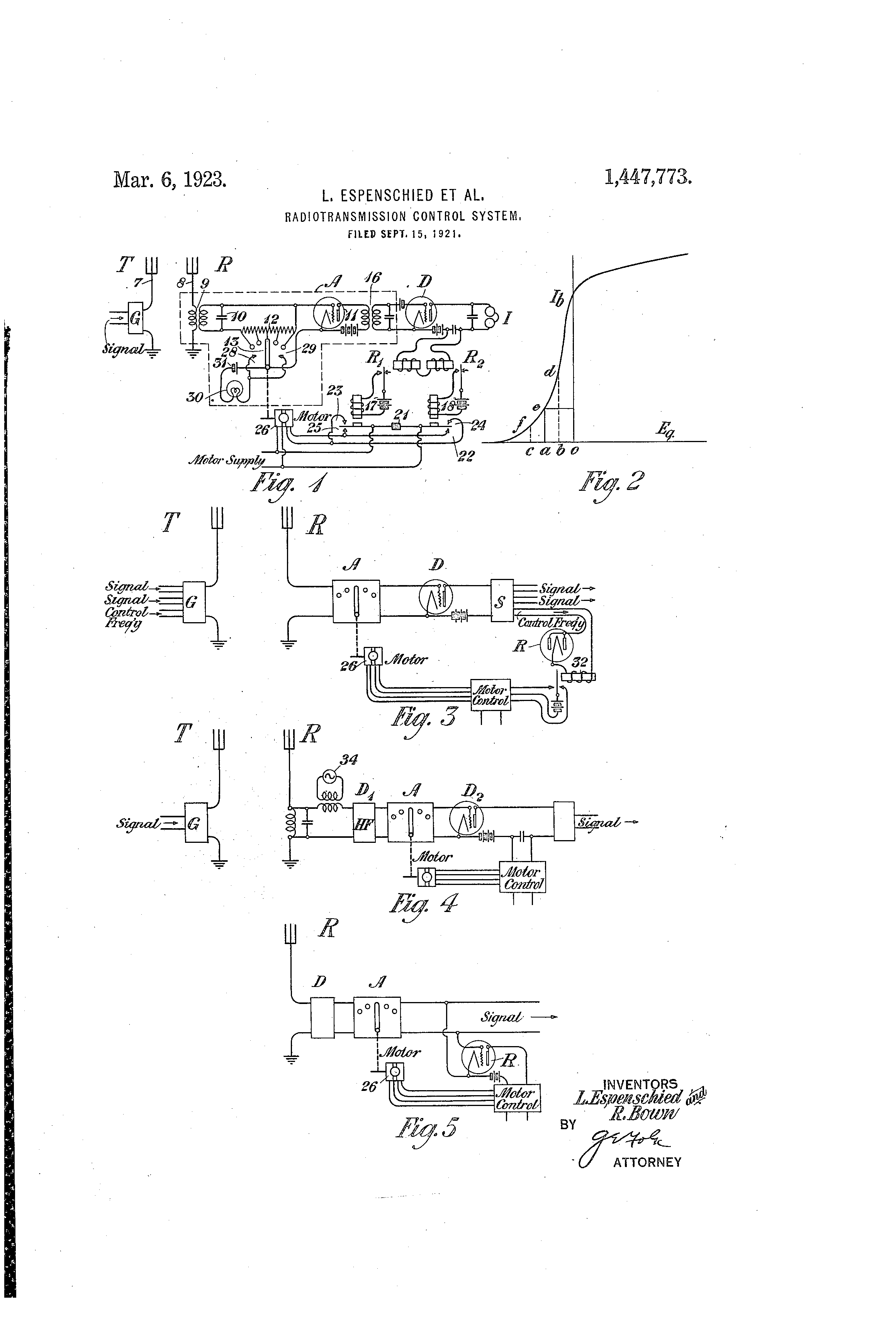
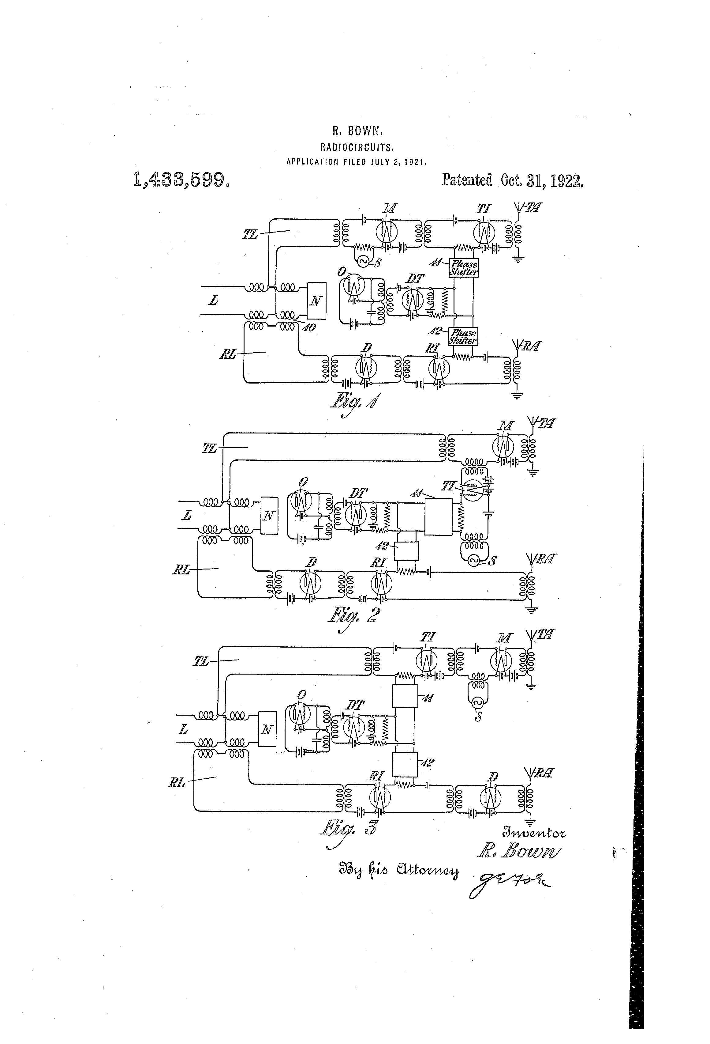
Additional related work: US1447773A (1923), US1433599A (1922).